Quickstart
Five minutes from import to a saved, styled, multi-backend plot.
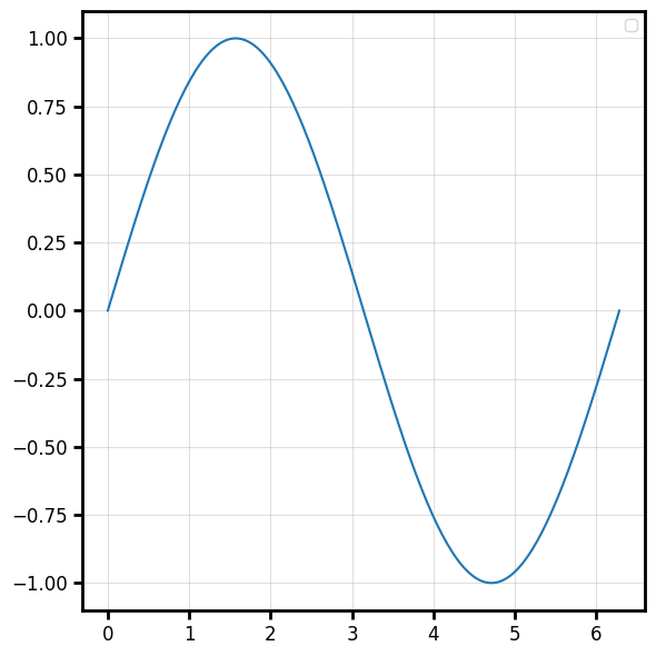
1. Your first plot
Every plot function returns a (fig, ax) tuple. matplotlib is the default backend, so
there is nothing to configure.
import numpy as np
import behaviz as bv

x = np.linspace(0, 2 * np.pi, 200)
y = np.sin(x)

fig, ax = bv.plot_line(x, y)
2. Switch the backend
The same call renders on a different engine. Set it once, globally.
bv.set_renderer("bokeh")        # or "seaborn", "matplotlib"
fig, ax = bv.plot_line(x, y)    # now an interactive bokeh figure
3. Plot from a DataFrame
Pass data= and reference columns by name (positional or keyword). See
Data input for the full resolution rules.
import polars as pl

x = np.linspace(0, 2 * np.pi, 100)
y = np.sin(x)
df = pl.DataFrame({"t": x, "signal": y})

bv.plot_line("t", "signal", data=df)

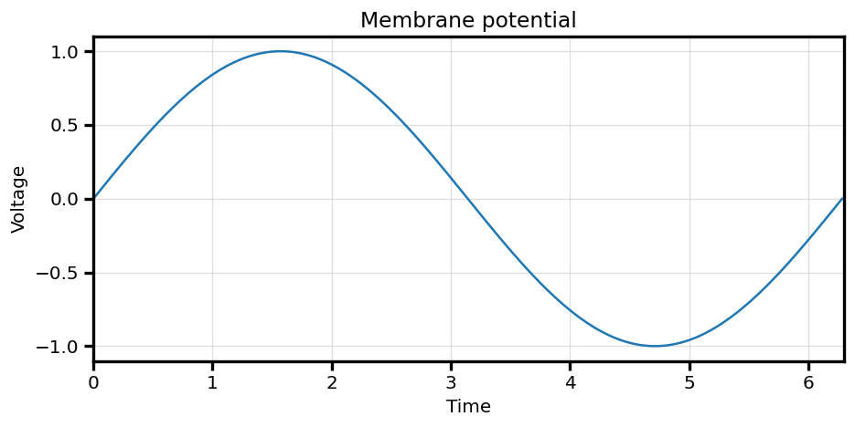
4. Style it with a spec
A PlotSpec describes the look. Chainable with_* mutators keep it
terse.
spec = (
    bv.PlotSpec()
    .with_title("Membrane potential")
    .with_xlabel("Time", )
    .with_ylabel("Voltage")
    .with_xlim(0, 6.3)
)

bv.plot_line("t", "signal", data=df, spec=spec)
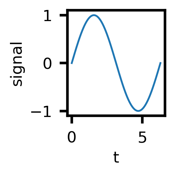
Or start from a preset:
spec = bv.load_preset("paper")
bv.plot_line("t", "signal", data=df, spec=spec)
5. One line per category
hue= colors and adds a legend; group= draws one series per category with no legend.
See Grouping.
x = np.linspace(0, 2 * np.pi, 100)
y = np.sin(x)
cond1 = np.zeros_like(y)

y2 = y + np.random.rand(100)
cond2 = np.ones_like(y2)


df = pl.DataFrame({"t":np.hstack((x,x)),
                   "signal":np.hstack((y,y2)),
                   "condition":np.hstack((cond1,cond2)),
                   })


df
bv.plot_line("t", "signal", data=df, hue="condition")

6. Save it
bv.save() dispatches on the active backend and the file extension.
fig, ax = bv.plot_line("t", "signal", data=df)
bv.save(fig, "figure.png")        # mpl/seaborn: png/svg/pdf...; bokeh: html/png/svg
Or use the canvas context manager to group several draws onto one axes and save in one shot:
with bv.canvas(spec=spec, save="figure.png") as ax:
    bv.plot_line("t", "signal", data=df)
    bv.plot_scatter("t", "signal", data=df)
Next
- Core concepts — the model behind the calls.
- Plotting overview — every plot type.
- The spec system — full styling vocabulary.